19-Sept, 2016 . Lab #7: Modeling Friction Forces

Lab #7:  Modeling Friction Forces

Dahlia - Ariel - Carlos

19-Sept-2016

The purpose of the lab#7 is to help students know how to calculate the static friction, kinetic friction on a level surface as well as on a sloped surface.
Part A: On a level surface
1- Static friction: 
Static friction describes the friction force acting between two bodied when they are not moving relative to one another. 
In this experiment, I worked with 1 block B1 with mass m stayed in table. Another mass B2 was hanging through a string and a pulley which was connecting with the block in the table.
then, I kept adding small mass onto B2 until B1 start moving. And I recorded the mass of B2.
Trail #2, I add another block on to the block B1, now I had 2 block on the table. I repeated adding small mass into B2 until 2 block on the table begin to move. and I recorded the mass of B2.
Trail #3 and trail #4, I did the same progress with 3 blocks and 4 blocks on the table.
This picture shown how I did trail #4

And this was what I recorded from 4 trials

trail #	Mass of block on table (g)	mass of hanging (g)
#1	180	90
#2	320	180
#3	496	265
#4	629	330

From the free body diagram of this situation, I had Fs=hanging mass*g
                                                                                  N=mass of block *g
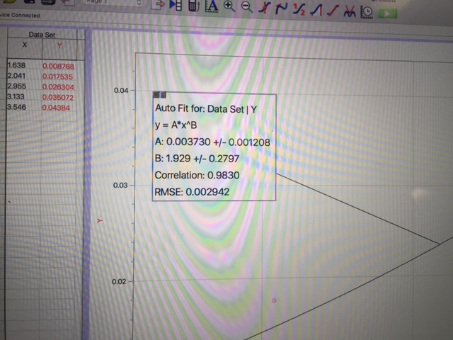
Moreover, Fs=μs*NThus, the slope of graph Fs and N was μs
based on the graph, the μs=0.532
2 - Kinetic friction
now, to find the kinetic friction, I had to give the blocks some forces.
I continued to do 4 trials with 4 different mass like part 1 above. then, I used a force sensor which was connected with log pro to read the value of force I provided for the block.
From the free body diagram of this situation, I had Fk=F-provide
                                                                                  N=mass of block *g
Moreover, Fk=μk*N
Thus, the slope of graph Fk and N was μk

This picture was when I did trial #3

Based on the graph, I could conclude the coefficient of kinetic friction was 0.26
Part B: On a sloped surface

1- Static friction: 
Now, I placed a block on a horizontal surface and slowly raised one end of the surface, tilting it until the block started to slip. then, I used the angle at which slipping just began to determine the coefficient of static friction between the block and the surface.

Then, I calculated them to find the coefficient of static friction

Thus, the μs=0.4
2- Kinetic friction: 
To find kinetic friction, I used a motion detector at the top of an incline steep enough that a block went down the slope

Through log pro, I got a=0.939 m/s^2
mass of the block was 0.18kg
the angle was 25.5 degrees
I used them to solve for μk

and the result was μk=0.37

15-Sept, 2016 . Lab #5: Trajectories

Lab #5: Trajectories

Dahlia - Ariel - Carlos

14-Sept-2016

The purpose of the lab#5 is to help students know how to calculate the initial velocity based on the distance of a steel ball go. Moreover, this lab also help students predict the impact point of the ball on an inclined board.

Materials: Aluminum "v-channel", steel ball, board, ring stand, clamp, paper, and carbon paper.

Part A: 
1. Set up:

we set up like this picture.
Then, we let the steel ball began to roll at the top of the aluminum "v-channel". This steel ball fell on the carbon paper. Thus, with the height of the table h, and the distance between the table and the carbon paper x, we needed to calculate the initial velocity of the steel ball.

we did this progress in 5 trials. this was the data we recorded after 5 times.

2. Analyzed data:
With the collected data, we calculated the value of distance x with uncertainty value:

thus, x=66.4± 0.3 cm
and the height of the table h = 90.0± 0.1 cm
so, we had:

Now, the initial velocity was 150.7 ± 0.7 cm/s

Part B:

Now, from part A,we know that the initial velocity was 150.7 ± 0.7 cm/s

with the known angle, we had to calculated distance d (as shown)

This were how we solved the problem.

Thus,we measured that distance d would be 79.6 cm.

then, we did an experience to check my work.

we measured the angle, and it was 48.6 degrees.

Then we let the steel ball move.

and we collected the result.

in 5 trials, our record was this.

This was not too bad. With the theoretical value for d was 79.6 cm, and the experimental values was shown, I could conclude that if I know the initial velocity and value of an angle, I could calculate the distance of the steel ball move along the slope.

12-Sept, 2016 . Lab #4: Modeling the fall of an object falling with air resistance

Lab #4: Modeling the fall of an object falling with air resistance

 Dahlia - Ariel - Carlos

12-Sept-2016

The purpose of the lab#4 is to help students know how to determine the relationship between air resistance force and speed.
Part 1: Collect data
We went to the building 13, and started to do the experience with dropping the coffee filters from a balcony.

Then, we used log pro to record data

We repeated drop 1,2,3,4,and 5 coffee filters at a time, thus, we had 5 videos in total.

Then we returned to class to analyze these video.

Part 2: Analyze 5 videos:

With log pro, we could record the relationship between the position of coffee filters vs time. Thus, with 5 video, we had 5 graphs.

* With 1 coffee filter:

* With 2 coffee filters:

* With 3 coffee filters:

* With 5 coffee filters:

* With 5 coffee filters:

To make them easier, I summarized them:

 Them I graphed them in log pro 

In which, x were the velocity of these coffee filters (the slope of period graphs)

                y were the force  (with 1 coffee filter, y=mg,

                                              with 2 coffee filters, y= 2mg, ....)

And because the mass of 150 coffee filters was 134.2 g; so the mass of 1 coffee filter was 0.8947 g.

and with g = 9.8m/s^2, I had graph:

This graph was the air resistance force.

Now, I had the equation of the air resistance force: F = 0.00373 v^1.929

Thus, 

The equation of acceleration, I got it from a free body diagram.

Part 3: Modeling the fall of an object including air resistance

Now, I opened a sheet of excel, and work the same way with the lab #3, the elephant problem

The interval of time was 0.01 s;
mass of 1 coffee filter was 0.0008947 kg;
gravity was 9.8m/s^2
k and n I got from the period part, part 2.
initial velocity was 0 m/s
initial time was 0s
in this sheet, time --------------------------A10=A9+$B$1
                     acceleration -----------------B9=($B$2*$B$3-$B$4*D8^$B$5)/$B$2
                     delta v------------------------C9=D9-D8
                     velocity ----------------------D9=B9*$B$1
Then, I filled them down until I had the constant velocity
*With 1 coffee filter:

Because delta t =0.01s was so small, and I had to filled down 315 rows to find the constant velocity, I changed the interval time into 1/30th. So, I had:
*With 1 coffee filter:

*With 2 coffee filters:

*With 3 coffee filters:

*With 4 coffee filters:

*With 5 coffee filters:

Now, I concluded that the bigger of the air resistance force, the larger of the speed we need.

12-Sept, 2016 . Lab #3: Non-Constant acceleration problem

Lab #3: Non-Constant acceleration problem

Dahlia - Ariel - Carlos

12-Sept-2016

The purpose of the lab#3 is to help students know how to use excel to calculate the distance of  an object can go (in a problem in which the acceleration of the object moving is non-constant and decreased over time.) or in other words, this lab will help students know how to calculate integration for kinematics by using excel.

The Problem:
A 5000-kg elephant on friction-less roller skates is going 25 m/s when its gets to the bottom of a hill and arrives on level ground. At that point a rocket mounted on the elephant's back generates a constant 8000 N thrust opposite the elephant's direction of motion. The mass of the rocket changes with time (due to burning the fuel at a rate of 20 kg/s) so that the 

m(t) = 1500 kg - 20 kg/s*t

Find how far the elephant goes before coming to rest. 

Analysis:

From the question, I knew that F(net) = 8000 N

                                                  total mass = 5000 + 1500 = 6500 kg

So, from the Newton's law, F(net) = m*a(t)

                                                   a(t)=F(net)/m

                                                         = -8000/(6500-20t)

                                                         = -400/(325-t)

 Now, to find velocity, I need to integrate a(t) with the bounded from 0 to t.

after I had velocity, to find the distance, I need to integrate v(t) with the bounded from 0 to t.

And the result of the integration was:

x(t) =[25-400ln(325)]t + 400[(t-325)ln(325-t)-t+325ln(325)]

To find how far the elephant goes before coming to rest, I needed to find the time at which the velocity of the elephant was zero.

From ∆v = 400ln(325-t)-400ln(325)=-25

=>t=19.69s

Plug this time to the expression for x(t), I had x = 248.7m

Thus, I open a sheet of excel and use this to find the time when the velocity become zero.

From this table, 

1. Column A: Time begins at 0, so start by setting time increased by 1 seconds (= A8+$B$5)

2. Column B: Since acceleration is not constant, so B8 (= -400/(325-A8))

3. Column C: a_avg = (a1+a2)/2 ----------------------C9 (=(B8+B9)/2)

4. Column D: ∆v = a_avg*t --------------------------- D9 (= C9*$B$5)

5. Column E: v = vf + vo. ------------------------------E9 (=E8+D9)

6. Column F: v_avg = (vf + vo)/2 ---------------------F9 (=(E8+E9)/2)

7. Column G: ∆x = v_avg*t ----------------------------G9  (=F9*$B$5)

8. Column H: xf = xo + ∆x -----------------------------H9 (=H8+G9)

Then, I filled down all of these columns until I saw the value of velocity was zero.

and I got velocity became zero when t =19s - 20s, and ∆x = 248 m

To make the result became more accuracy, I changed the change of time become 0.1s

Now, I got the better value. Velocity became zero when t =19.6s, and ∆x = 248.69 m

Conclusion:

1. the result I got from doing the problem analytically and doing it numerically was the same. Velocity became zero when t =19.69 s, and ∆x = 248.7 m

2. From the problem, when I use t=1s, the result would not accuracy than 0.1s. From the above table, I could see the distance did not change so much in 19.6, 19.7, and 19.8s, that mean the time 0.1s was small enough.

08-Sept, 2016 . Lab #6: Propagated Uncertainty Calculations

Lab#6: Propagated Uncertainty Calculations

Dahlia - Ariel - Carlos

08-Sept-2016

The purpose of this lab is to help students calculate some values of uncertain members. In the real world, we can not do any experience in one time, and assign the result as its value. Indeed, we have to do so many time, and of course, we cannot receive the same result in every single trial. Knowing how to calculate uncertainty value is very necessary skill for students.
1. Set up:

First, we had two different objects A and B:

And we need to measure their diameters, their lengths, and their weights.

To measure them, we used a very special tool:

and then, this was what we got:

2. Calculate:

With these data, we could calculate the uncertainty value of the density(mass / volume) of two objects based on formula:

ρ = 4m/πd²h.

and 

Apply the formula, I had answer:

Thus, with object A, density would be 2.84±0.046 g/cm^3

object B would be 7.007±0.1149 g/cm^3

07-Sept,2016 . Lab #2: Free Fall Lab

Lab #2: Free Fall Lab

Dahlia - Ariel - Carlos

08-Sept-2016

The purpose of this lab is to examine the validity of the statement: in the absence of all other external forces except gravity, a falling body will accelerate at 9.8 m/s^2. The second purpose of this lab is to help students know a bit about Excel such as how to enter data, how to fill down, or how to graph from  a certain set of data.

Part 1: Free fall

Set up:
Use the apparatus to record the series of dots which was represented to the position of the falling mass every 1/60th of a second
These dots was in a piece of paper tape.
Measure and record the position of each dot.

Data:
These pictures shown the progress we recorded the position of each dots and received data.

Then, we measured the position of each dots.

After that, we recorded them into Excel.

In this table:
- Column "time" shown 1/60s, 2/60s, 3/60s, and so on.
- Column "distance" shown the position of each dot.
- Column "delta" shown the position of each dot related to period dot.
                       Delta = position of dot number #(n+1) - position of dot number #n
- Column "Mid-interval time" shown the time for the middle of each 1/60th second interval.
- Column "Mid-interval speed" shown the average speed in each interval.

After that, we graphed our data.

Analysis:
1.
For constant acceleration, we can see that the velocity in the middle of a time interval is the same as the average velocity for that time interval.

2.
The value of g was the slope of the line of speed vs. time.

With v =925x + 45
        a= v' = 925
My result was lower that expected result.

3.
The value of g was the second derivative of the curve of position vs. time.
With y= 465 x^2 + 43x + 0.28
         v= y' = 930x+43
         a = v' = 930
My result was lower that expected result.

Conclusion:
From the analyzed data, I could see that the difference between each dot and the speed of them in the interval 1/60th second were increased patently.

From the fact, the gravity is 9.8m/s^2, but my group answer was 9.25m/s^2. This happened because of some reasons such as the frictions, the mistakes when we measured the positions of dots.
The absolute difference was 9.25-9.8=-0.55m/s^2.
The relative difference was (9.25-9.8)x100%/9.8 = -5.61%

Part 2:Errors and uncertainty

When doing this experience, Our group result was 9.25m/s^2; however, each group in the class received different results. The below table was what the class had.

After that, we entered these values into a sheet of Excel.

In which 948.25 was the average of g; 672.6875 was the average deviation value; and 25.9362 was standard deviation value.
To get the dev. from the mean, we used formula

From what we had, we received result:

However, the lowest value in our result was 893, and the acceptable value was 896-1000 m/s^2. Thus, 983m/s^2 became an "outlier", and we crossed out this value to make the result became more creditable.
This was what we had

And the value was 956 ± 32 m/s^2

1. From the class' values, I could realize that our value was lower than the real value.
2. Compare to the accepted value, I also saw that our value was lower than the real value.
3. Actually, there was no pattern in the class' value of g. There was different not because of the progress was wrong; there was different because of some errors called systematic errors and random error.
4. Random error was variation. We can not attribute the anything in particular.
    Systematic error came from our assumption about experiment, which are not true.

Conclusion:
In the real world, we can not do any experience in one time, and assign the result as its value. we have to do so many time, and of course, we cannot receive the same result in every single trial. Therefore, the uncertainty value will make the result we come up with become more acceptable. The lower of percent error and uncertainty value, the higher of creditable result.